At the end of 2024, we held an online panel on RL and control, Podcast: RL + Control—Bringing Robot Reliability Closer to 99.9x%. One guest made a point about the different approaches to RL: “When we talk about reinforcement learning, we need to specify which kind we mean. Is it sim-to-real model-free reinforcement learning? Learning a world model—the very popular model-based reinforcement learning approach? Or model-free reinforcement learning directly in the real world? I think these approaches differ quite substantially. Then there is offline reinforcement learning: when you have a lot of demonstration data, you can do offline RL as well as imitation learning. The differences between kinds of RL may be greater than the differences between RL and control.”
That observation made me want to put together an in-depth introduction to reinforcement learning and robotics. In fact, RL + Robotics was the starting point for Smart Note’s series on embodied intelligence in June 2023. A year and a half ago, inspired by Covariant’s approach, discussed in Covariant: The AI-for-Robotics Unicorn Founded by Three Chinese Researchers, I collected learning resources online about combining RL with robotics. The widely circulated AI + Robotics Chinese Researcher Map was even called the RL + Robotics Chinese Researcher Map in its first draft. A year and a half later, I wanted to understand how the many different RL algorithms fit into robotics today.
For this article, I interviewed two scholars whose work offers valuable perspectives on RL: Professor Weinan Zhang of Shanghai Jiao Tong University and Dr. Yunlong Song of the University of Zurich. I also brought together views expressed by Qiuguo Zhu, Guanya Shi, Zongqing Lu, and Jianlan Luo in Podcast: RL + Control—Bringing Robot Reliability Closer to 99.9x%. My original plan was to synthesize everything into a set of conclusions. But I did not want my editing to erase the interviewees’ reasoning or lose information, so I have kept the interview format, as usual. Some answers overlap; I hope readers will bear with the repetition.
I hope this long introduction to RL + Robotics—more than 10,000 Chinese characters in the original—is useful to you.
Original article outline
Contents
👇
Part One: Interview with Weinan Zhang
1. Value-based RL vs. policy-based RL
2. Online/offline RL vs. on-policy/off-policy RL
3. Model-based RL vs. model-free RL
4. Q-learning
5. Sim-to-real RL
6. Teacher–student learning
7. RL and manipulation
Part Two: Interview with Yunlong Song
8. Classifying RL
9. Value-based RL vs. policy-based RL
10. Are on-policy and off-policy subcategories of policy-based RL?
11. Model-free RL vs. model-based RL
12. How RL differs across drone control, locomotion, and manipulation
13. Perception in drone flight and manipulation
14. RL and MPC for drone control
15. Trends in drone research and applications
16. Differentiable simulation and locomotion
Part Three: Podcast: RL + Control—Bringing Robot Reliability Closer to 99.9x%
Part One: Interview with Weinan Zhang
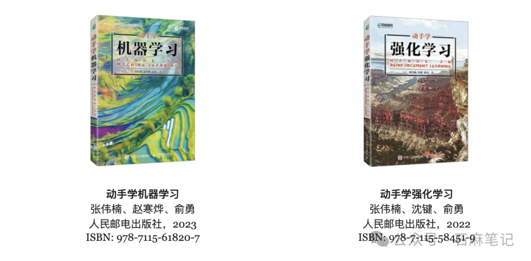
Dr. Weinan Zhang is a professor, doctoral supervisor, and associate department head in Computer Science at Shanghai Jiao Tong University. His research includes reinforcement learning and data science. At the time of this article, his work had received more than 20,000 Google Scholar citations. He earned his bachelor’s degree from SJTU’s ACM Honored Class in 2011 and his PhD in Computer Science from University College London in 2016. He has coauthored the textbooks Hands-on Reinforcement Learning and Hands-on Machine Learning. These biographical details describe the original interview period.
During our conversation, I was struck by Professor Zhang’s deep understanding of reinforcement learning and his ability to explain complex ideas vividly and clearly. The following is our discussion of how to classify RL.
There are many ways to classify reinforcement learning. Broadly, we can distinguish value-based and policy-based RL; online and offline RL; on-policy and off-policy RL; and model-based and model-free RL.
1. Value-based RL vs. policy-based RL
Value-based RL uses repeated interaction between an agent and its environment to estimate expected cumulative return. That expectation is the value. By learning a value function, the agent evaluates how good different states or actions are and uses those evaluations to choose actions. Q-learning, SARSA, and DQN are examples of value-based reinforcement learning algorithms.
Value-based reinforcement learning guides an agent’s decisions by learning a value function. Its central idea is to evaluate the value—the relative “goodness”—of each state or state–action pair and choose actions accordingly. In this framework, the policy is not optimized directly through policy parameters. Instead, the agent learns how valuable each state, or each action in a given state, is, and derives its action choices from those evaluations.
A value function estimates the expected cumulative future reward an agent can obtain starting from a particular state. There are usually two forms. A state-value function estimates the expected return from a state. An action-value function estimates the expected return from taking a particular action in that state and then following a policy.
Policy-based RL optimizes the policy directly. A pure policy-gradient method does not require a learned value function; REINFORCE is a familiar example. Pure policy-only methods are less common in the settings we are discussing.
Policy-based RL maximizes cumulative return by adjusting the agent’s policy parameters. Rather than choosing actions only through value estimates, it directly learns a parameterized policy, usually a neural network. A policy is the rule for selecting an action in a state; it can be deterministic or stochastic. [Terminology note: many policy-based methods also learn a value function to assist optimization. The absence of a value function describes the pure policy-only case, rather than every policy-based method.]
There are also methods that combine a policy and a value function, learning and optimizing both. Familiar examples include A3C (Asynchronous Advantage Actor-Critic), A2C, PPO (Proximal Policy Optimization), TRPO (Trust Region Policy Optimization), and DDPG (Deep Deterministic Policy Gradient). These are commonly implemented within an actor–critic framework. Such methods are particularly useful for high-dimensional states and actions, including flexible behaviors in continuous action spaces. [PPO and TRPO are policy-optimization methods often paired with a value-function critic; that implementation choice should not be mistaken for a requirement in their definitions.]
2. Online RL vs. offline RL vs. on-policy RL vs. off-policy RL
The main difference between online and offline RL is whether training includes new interaction with the environment. Online RL collects experience through ongoing interaction; offline RL trains on data collected in advance.
In the online setting, both on-policy and off-policy learning are possible. The distinction concerns whether the data used for learning comes from the policy being learned. On-policy methods use data generated by that policy; off-policy methods can learn from data generated by a different policy. [The original describes both as belonging to online RL. More precisely, this is a separate classification axis: offline RL also learns from off-policy data.]
The distinction I am making here is between online learning, which continues to interact with the environment, and offline learning, which works with previously collected data. Modern deep offline RL became especially prominent around 2018–2020. With a fixed dataset, training can proceed without further interaction and may be faster when interaction is the bottleneck. In the online implementations I have in mind, on-policy methods collect fresh experience, while off-policy methods retain experience in a replay buffer. [Clarification: offline or batch RL predates 2018. Neither continued interaction nor a replay buffer defines off-policy RL; a buffer is a common implementation. On-policy algorithms such as PPO may also reuse their current batch for several optimization epochs.]
I often use an analogy to explain this. On-policy learning is like washing your hands under a running tap. The water passing over your hands represents data. Once it has passed through, it drains away rather than being used again. If the water flows too quickly, much of it may be wasted.
Off-policy learning is more like placing a basin under the tap. You collect the water in the basin and reuse it rather than washing directly under the running stream. Once the basin is full, the oldest water spills out. In the replay-buffer version of off-policy learning, collected data is stored and can be reused at different times.
Offline learning goes one step further: there is no running tap at all, only a basin already filled with water. You keep washing your hands in that water. Training does not depend on new, real-time interaction with the environment. You collect the data first and then reuse it for learning.
The environment and task shape which approach is practical. In a game, the engine may let you play whenever you want and generate effectively unlimited experience, making on-policy learning feasible. If data arrives so quickly that much of it would otherwise be wasted, a “basin”—a replay buffer—can help, and you may choose online off-policy learning. Conversely, when collection is very expensive, every sample matters. A factory floor is an example where you might instead train offline on the available data.
As a rule of thumb: if data is scarce and difficult to obtain, consider offline RL. If data is obtainable but valuable, consider off-policy learning and storing it in a replay buffer, where a full buffer may discard its oldest entries. If data can be generated continuously and cheaply, on-policy learning may be practical. These are resource-based heuristics, rather than exclusive rules about which algorithm a task permits.
3. Model-based RL vs. model-free RL
Historically, many approaches used a model of the environment. Once a model is available, an agent can explore possible outcomes within it, perform dynamic programming, or generate simulated experience without disturbing the real world. Environments such as mazes and Go provide familiar examples where a model can support planning. Here, “model” generally means a model of the environment’s dynamics, not the neural network representing the policy or value function. Model Predictive Control (MPC), for example, uses dynamics to plan. [A perfect or complete model is not required for model-based RL, and not every RL algorithm applied to a maze or Go is model-based.]
An environment model usually describes two things: state transitions and rewards. Modeling the dynamics or transition function is especially common. Once the model is available, the agent can use it for dynamic programming. The central idea is to use the model—whether given or learned—to make decisions and plan.
The difficulty is that an inaccurate environment model can produce poor results. Model-free approaches instead rely more directly on experience, without first constructing a detailed dynamics model. Richard Sutton helped establish this tradition, and David Silver later contributed to its development in deep RL. Q-learning is a typical example: it learns an action-value function, or Q-function, that helps identify good actions in each state. It does not need an explicit dynamics model; it learns from transitions containing a state, action, reward, and next state. [The original attributes the invention of model-free RL to Sutton and Silver and lists only three transition elements. Model-free RL has a longer history, and Q-learning also uses the next state.]
Concrete learning algorithms implement this process, including temporal-difference (TD) learning. TD methods include both on-policy and off-policy approaches.
4. Q-learning
Q-learning is an off-policy method: it can learn from data generated by a behavior policy different from the policy it is trying to improve. For example, the agent can use experience collected by other policies or by earlier versions of its policy. This offers flexibility and allows learning from several sources of experience. An on-policy method, by contrast, learns about the policy generating its current data.
One advantage of ordinary Q-learning is that its update does not require an explicit importance-sampling correction for the behavior policy. Some off-policy algorithms correct for the difference between the policy that generated the data and the target policy. Q-learning’s particular update can use other policies’ transitions without that correction. [This does not mean every other off-policy algorithm requires importance sampling.]
In practice, Q-learning can learn from experience without a complicated environment model. Given states, actions, rewards, and next states, it learns a Q-function from which a policy can be derived. Explicit transition probabilities and reward distributions are unnecessary. Under the appropriate tabular-learning assumptions, it can converge to the optimal action-value function; arbitrary datasets and deep-network approximations do not carry the same blanket guarantee.
Chris Watkins introduced Q-learning in 1989. It learns from interaction without requiring an environment model. Richard Sutton and other researchers helped develop and popularize this family of methods through the 1990s and early 2000s. In 2013, DeepMind’s Volodymyr Mnih and colleagues, including David Silver, introduced the Deep Q-Network (DQN), combining Q-learning with deep neural networks. DQN became a landmark in deep reinforcement learning: it enabled Q-learning to work with high-dimensional inputs such as images rather than only simple state representations. [The original credits DQN to Silver alone; it was a collaborative paper led by Mnih.]
As the interview recounts it, while working at UCL, David Silver repeatedly tried to persuade companies in London to adopt model-free RL, initially with little success. People were skeptical of learning directly from data without modeling the environment. Particularly when data was limited, the familiar approach was to describe the environment with a model and solve the resulting problem through dynamic programming. This is the speaker’s recollection, rather than an independently verified biographical account.
In that account, the arrival of much larger datasets made these data-driven approaches increasingly feasible and reliable. Silver did not receive immediate widespread recognition after returning to UCL, but continued pursuing model-free learning and developing the approach.
The rise of deep learning then brought major breakthroughs. A deep network’s expressive power allowed algorithms such as Q-learning to tackle more complex tasks. Representing the Q-function with a convolutional neural network lets it learn from large amounts of data and be optimized at much greater scale. AlexNet illustrates the broader deep-CNN breakthrough mentioned in the interview; the original DQN used its own smaller CNN, rather than AlexNet itself.
This represented a major shift from methods centered on hand-built environment models and limited experience. Deep Q-learning could learn and improve directly from large amounts of data, achieving success on tasks such as Atari games. It marked an important step forward for deep reinforcement learning and expanded the kinds of problems these methods could address.
Both model-based and model-free methods have strengths and weaknesses. Model-based methods use simulation and planning to anticipate future states; model-free methods lean more heavily on learning from accumulated experience. With advances in deep learning, model-free methods such as Q-learning became especially influential in complex, high-dimensional environments.
5. Sim-to-real RL
Learning robot policies brought renewed attention to sim-to-real transfer. Earlier attempts to use RL for robot locomotion or manipulation often struggled, and relatively few researchers pursued them at scale. I would emphasize two reasons. [The original suggests that sim-to-real problems did not previously exist; transfer between simulation and reality was already a longstanding robotics problem. Learned policies made it especially prominent in this context.]
First, RL can require large amounts of experience. Trial-and-error learning depends heavily on interaction data that reveals the consequences of actions. Supervised learning can use labeled examples directly, and unsupervised learning can extract patterns from unlabeled data. RL needs experience informative about rewards and transitions. That experience may be collected during training or supplied in advance for offline RL; not every RL algorithm requires new online interaction.
Second, deployment has to respect the physical realities of a robot. A policy that appears effective in simulation may fail on hardware if training and transfer are inadequate, particularly for walking, running, and jumping. Insufficiently trained policies may repeatedly damage equipment, and breaking ten or even a hundred robots is unacceptable. These costs make simulation a natural training environment for such tasks. They do not rule out real-world RL under suitable safety and data-collection arrangements.
Simulators have limitations too. They operate through specified equations and cannot reproduce reality perfectly. Contact and collisions—for example, a robot’s leg hitting the ground—can be particularly difficult to simulate accurately. This mismatch is called the reality gap.
Sim-to-real techniques help a policy trained efficiently in simulation cross that gap. Two major approaches are domain randomization and domain or policy adaptation. Domain randomization changes environment parameters across many dimensions during training, exposing the policy to a broad range of conditions. If it remains effective across that variation, it may be more robust in reality. This is widely used for learned policies on platforms such as quadrupeds and robot arms. Adaptation incorporates real-world data to adjust the policy to the physical environment. In the example given here, roughly 95% of training is simulated and 5% uses real data; these percentages are illustrative, not a standard ratio. Collecting real data remains difficult: noise and poor-quality observations can undermine the policy. [The original’s claim that most quadruped and industrial robots use domain randomization should be read in the context of learned sim-to-real policies, not the entire industrial robot population.]
Some adaptation approaches collect real-world data and use it to adjust the simulator’s parameters, bringing simulation closer to reality. This kind of system identification does not eliminate every problem, but it can be comparatively reliable and is widely used.
6. Teacher–student learning
With domain randomization, one policy has to work in many environments. Consider a “blind” quadruped: it cannot see the terrain half a meter ahead and has to feel its way forward. It does not know exactly what terrain it is on or what will happen after its next step. Its local observations mostly come from proprioceptive sensors on the body and four legs, so they provide only incomplete information. The interview calls the terrain “nonstationary”; the issue illustrated here is primarily partial observability, which does not by itself mean that the underlying dynamics change over time.
But in simulation you can “cheat”: you can inspect every nearby grid cell and its terrain. The environment becomes transparent, making it much easier to train a policy quickly. We call that extra information privileged information. It is like revealing the whole map in a game, so learning where to step becomes easier.
We first train a teacher policy with that broader information, then distill it into a student policy that sees only local observations. In practice, the student may not know why a particular step is appropriate, but it learns the action the teacher would take. The teacher can see a rock ahead and knows that the next step should be placed farther back; that is the basic idea.
Usually, the teacher learns first. Once trained with privileged information, it supervises the student: “Move in this direction now,” or “Make this movement then.” The student learns to reproduce the teacher’s behavior through a regression-style objective.
7. RL and manipulation
If a robot’s task is essentially path planning followed by path execution, it may not need RL. Many computer-vision colleagues first use vision to understand the environment, then plan a path and execute it. In that setting, there may be little need for additional, more complex manipulation learning.
A key question is whether interaction with the environment requires high-frequency, real-time dynamic control. If it does not, planning a path and executing it may be enough.
Take folding clothes. In a largely quasi-static approach, the fabric hangs naturally from the two arms, and gravity brings it together as the arms move. Within that approximation, the precise movement speed is not central to the folding process: whether the arms move somewhat faster or slower, the cloth still hangs below them. This is what I mean by “static execution.”
If the task involves flinging the cloth into the air, however, the dynamics matter. That is a setting where I see a strong role for RL. Quadruped walking is another example: fast, coupled leg movements cannot be handled simply by independently planning and executing one path for each leg. Locomotion is a different kind of problem, which helps explain why dynamic control has been such an important research direction. [The speaker’s wording that these tasks “need RL” expresses a preference; dynamic tasks can also be solved using other control methods.]
Now consider manipulation with a simple gripper. A basic “close once” action may involve fewer changing variables and lower dynamic demands. You might only care about commanding 0 or 1—release or grasp—rather than controlling every detail of the process. Many early manipulation settings look like that, and may not need RL or particularly elaborate learning.
As dexterous hands become more common, I expect RL to play a larger role in finely controlled, flexible movements. Those intricate behaviors often require high-frequency dynamic control far beyond a simple binary command. This is the speaker’s view of RL’s promise, not a claim that all dexterous manipulation must use RL.
Part Two: Interview with Yunlong Song
Dr. Yunlong Song conducted his PhD research under Professor Davide Scaramuzza in the Robotics and Perception Group, within the University of Zurich’s Department of Informatics and the joint UZH–ETH Zurich Department of Neuroinformatics. During his PhD, he visited MIT’s Biomimetic Robotics Lab and worked with Professor Sangbae Kim. Before that, he earned his master’s degree at TU Darmstadt under Professor Jan Peters. [The original biography simultaneously calls him “Dr.” and a doctoral student; his personal page records his PhD in 2024. The description here preserves his doctoral affiliations without implying he remained a student in January 2025.]
(Several of Yunlong’s mentors are renowned researchers. Davide Scaramuzza is a leading figure in drone autonomy and learning; Sangbae Kim is well known for MIT Cheetah. The research lineage around Jan Peters and his mentor Stefan Schaal is an important branch of European robot learning. Peters also coauthored the influential Reinforcement Learning in Robotics: A Survey, together with Jens Kober and J. Andrew Bagnell. The original identifies Peters as the corresponding author; the paper’s author list establishes the coauthorship.)
Before joining UZH, Yunlong did extensive theoretical work, then explored applying reinforcement learning to drone control. During his PhD, he also encountered traditional control, particularly optimization-based optimal control, found it fascinating, and studied it systematically. His doctoral research grew from these two foundations—optimal control and reinforcement learning—into further methods and applications. He developed Flightmare and a pioneering RL policy that pushed highly agile drones toward their physical performance limits. Before our discussion of RL classifications, let us watch a drone-racing demonstration using his reinforcement-learning approach.
8. Classifying RL
At the theoretical level, there is not that much entirely new material; it is often “old wine in new bottles.” Traditional RL discussed many of today’s classifications before deep learning arrived. The classification depends on the angle from which you look at the problem.
At the broadest level, we can distinguish deep reinforcement learning from non-deep reinforcement learning. The difference is whether deep-learning techniques are used.
Another distinction is value-based versus policy-based RL. AlphaGo is an example involving deep value learning, while policy-based deep RL is especially common in robotics. Hybrid methods combine value and policy learning. [AlphaGo is not a purely value-based algorithm: it combines policy networks, a value network, and tree search. The original’s example should be understood with that qualification.]
A third classification concerns on-policy and off-policy learning. I am not sure whether your reference to online and offline means on-policy and off-policy, but the latter is a common distinction. “Online” commonly refers to collecting new interaction data and updating parameters during training; in practice, updates need not happen continuously at every interaction. On-policy means that data used to update the policy comes from the policy being learned. Off-policy means that the data comes from other policies or sources. Online/offline and on-policy/off-policy are related but different axes.
Each has advantages and disadvantages. On-policy methods commonly need more samples because they rely on experience from the current policy. Off-policy methods can reuse historical experience and experience collected by other policies, often improving sample efficiency.
Many familiar value-based algorithms, such as DQN, are off-policy, while many policy-optimization algorithms, such as PPO, are on-policy. The on-policy/off-policy distinction therefore classifies learning by the relationship between the policy being learned and the source of its data.
A fourth distinction is model-based versus model-free RL. A model-free method optimizes from experience without explicitly learning or using an environment model for planning. A model-based method first learns or constructs an environment model, then uses it to generate predicted experience, plan, or optimize a policy.
We can also distinguish reinforcement learning from inverse reinforcement learning (IRL). IRL focuses on inferring a suitable reward function from behavior data, addressing the difficulty of specifying rewards in RL.
In the robotics settings I work on, we often use on-policy algorithms such as PPO. Robot control signals usually lie in continuous action spaces, for which explicit policy optimization is convenient. Value-function methods are often associated with discrete actions, such as board-game moves. This is a tendency, not a strict division: both families can be adapted to discrete or continuous control.
Around 2019, better hardware, including GPUs, and accessible open-source tools made PPO easier to use. With enough suitable data, it could deliver strong results. Stable Baselines is an example of such tooling. [The original credits Stable Baselines to OpenAI; it is a separate project descended from OpenAI Baselines. More data alone does not guarantee good performance.]
Consequently, more robotics research adopted policy-based methods such as PPO. Previously, a lab’s choice often depended on its resources and existing code. PPO has become something like a standard choice in the simulation-heavy robotics work I am discussing. Off-policy methods such as SAC (Soft Actor-Critic) can be more sample-efficient, but achieving strong practical performance is not always straightforward. A GPU can generate large quantities of experience, yet an implementation may struggle to process it fast enough, leading to longer training times. In other words, fewer required samples do not necessarily mean shorter wall-clock training, which can limit adoption in these settings. [SAC combines a stochastic actor with learned critics; the original calls it value-based, but it is more precisely an off-policy actor–critic method. These speed and adoption observations are context-dependent, not universal rankings.]
9. Value-based RL vs. policy-based RL
My understanding is that the distinction largely concerns how the learning objective is optimized. In a value-based method, we start from the Bellman equation and commonly minimize a Bellman error or TD error to learn the value function.
Policy-based methods instead use policy gradients to improve expected return. From this perspective, value learning minimizes an error such as a TD error, while policy optimization directly maximizes an expected cumulative-return objective. These are different optimization routes toward better behavior, rather than necessarily different ultimate goals.
We should not rigidly equate value-based learning with discrete control and policy-based learning with continuous control. SAC, for instance, handles continuous control through its actor and critics, while policy gradients also work in discrete action spaces.
Historically, policy-based methods were especially associated with continuous actions and value-based methods with discrete actions. Neural-network function approximation lets us tackle many different settings, so the old boundary has become increasingly blurred.
10. Are on-policy and off-policy subcategories of policy-based RL?
No. On-policy versus off-policy is a broader classification, not a distinction confined to policy-based or value-based methods. Value-based learning also includes on-policy algorithms, such as SARSA.
On-policy learning uses experience from the policy being learned. After optimizing on the current collection of data, these methods typically move on to fresh experience rather than retaining an unrestricted historical replay dataset. This often increases sample requirements. An algorithm such as PPO can nevertheless reuse the current batch over multiple update epochs.
Off-policy learning can use experience collected by other means, including human demonstrations, older Q-function-derived behavior policies, or other policies. Many implementations use a replay buffer and repeatedly sample it for updates, improving data reuse. That can improve sample efficiency, although it need not improve training speed. A replay buffer is a common feature, not the definition of off-policy learning.
Off-policy algorithms are common among value-based methods, but “value-based” does not mean “off-policy,” and “policy-based” does not mean “on-policy.” They describe different dimensions of an RL algorithm.
11. Model-free RL vs. model-based RL
The distinction is fairly direct: does optimization explicitly use an environment model? If it does, it is model-based; if it does not, it is model-free.
There is some subtlety in what “using a model” means. Many model-free methods collect experience in a simulator. In the convention I am using, they remain model-free if the simulator supplies sampled transitions rather than being explicitly used for model-based planning or differentiation in the policy update.
MPC uses an explicit model to predict future states or compute optimization information, then uses those predictions to select actions. It is therefore clearly a model-based control method. That does not automatically make every MPC controller a reinforcement-learning algorithm.
There is also a distinction between MPC and other model-based approaches concerning where the model comes from and how it is used. MPC often starts with known or first-principles dynamics. Some model-based RL methods instead learn dynamics from data, for example with a neural network. MPC can also use learned models; the categories overlap.
Model-based methods employ different optimization strategies. They might use a model to sample or predict trajectories in an MPC-style receding-horizon loop, or use gradient-based or gradient-free search. The important question is exactly how the environment model enters policy optimization or action selection.
Some model-based methods learn more than dynamics: they may also learn a reward model and a value function. Papers such as Dreamer and PlaNet illustrate learning latent dynamics and rewards and using them for decisions. [Their components differ: Dreamer learns behavior with an actor and value estimates through imagined trajectories, whereas PlaNet is primarily a latent-model planning method. The original groups them together as learning all three components.]
A learned model alone does not tell us which action to take. We still need a decision method. A common approach is MPC-style planning: sample or predict candidate action sequences, evaluate their longer-term returns, and select an action. This adds planning and decision-making on top of the model. Other approaches, including Dreamer, use the model to train a policy rather than conducting this search at every real-world step.
If we only fit a value function without learning dynamics, the fitting operation looks like regression; that alone does not distinguish model-based from model-free learning. We also need a way to choose or improve actions. In the approach I am describing, optimization then determines the action or updates the policy. [Learning a value function through Bellman or TD updates is itself a core part of RL, and RL can be offline. The original’s statement that RL begins only with online action optimization is too restrictive.]
Authors do not always distinguish model-based methods, model-free methods, and RL optimization carefully. Some work is labeled model-based even though its actual use of the model fits another convention, or its learning procedure is not really RL. Such terminology can mislead readers, so it is worth examining the actual algorithm rather than relying on its label.
In locomotion, my estimate is that at least 80% of the stronger results at the time came from model-free methods. Learning accurate dynamics is difficult; even with a learned model, optimizing the policy or actions through it remains challenging. In my experience, this has often limited the performance of model-based approaches. The 80% figure is the interviewee’s estimate, not a systematic benchmark or census.
Some model-based methods also learn rewards and value functions. Each learned component can introduce error, and those errors may compound, making performance less stable than direct model-free learning. Model-based methods can potentially use fewer environment samples, but the optimization may be harder, particularly when deciding how to extract good actions from the learned model.
The ideal vision for model-based RL is to learn an environment model from a modest amount of data and gain three benefits. First, reduce the sim-to-real gap by training the model on real experience rather than writing a simulator by hand. Second, reduce sample requirements: once the model exists, adapting a policy might need only a small amount of new data. Third, reuse the model when the reward or task changes, greatly improving efficiency.
In practice, those benefits have not always been fully realized. Many approaches still generate training data in a hand-built simulator, which inevitably differs from reality. Deploying the resulting policies on physical systems brings further difficulties. Bridging that gap remains an important open problem.
12. How RL differs across drone control, locomotion, and manipulation
I have not personally carried out a manipulation project, so these are subjective observations. Manipulation differs fundamentally from drone flight and locomotion in several respects.
First, the object of attention differs. A drone or locomotion controller focuses heavily on the robot’s own state, such as its attitude and joint angles. Terrain and other environmental factors matter too, but manipulation places even greater emphasis on the external environment. It requires understanding the arm or hand’s pose as well as the objects around it.
Second, object diversity matters. Introducing a cup or tool with a different shape, weight, or material can substantially change the manipulation strategy. General-purpose manipulation therefore needs broad understanding of geometry, weight, and other physical properties. Some people argue that solving truly general manipulation would address a core problem in AGI, because it requires such strong perception and understanding of unfamiliar objects. This is an interpretation of the challenge, not an equivalence between manipulation and AGI.
Third, perception is central. Inferring an object’s shape, weight, and material and using that information to plan a grasp involves more than a simple control problem. For a straightforward pick-and-place task, if the relevant properties are already known, executing the movement may be relatively simple and may not need RL or a complex neural network.
Fourth, there are high expectations for large models. People hope they can provide higher-level environmental understanding, including reasoning about object properties and the scene. If that understanding becomes reliable, the grasping action itself may be easier to execute.
For manipulation, then, the difficulty is not confined to control. Accurate perception and modeling of the environment, especially unfamiliar objects, are crucial. Training only in simulation still leaves many unexpected real-world variations and object differences. That is an important reason why general-purpose manipulation remains challenging.
Manipulation also requires long-horizon task planning. Cooking in a kitchen or tying a shoelace requires decomposing a task into several steps and arranging them in the right order, in addition to perceiving and understanding the objects.
These tasks are harder to express mathematically and reward than flying a drone from A to B. Turning an abstract process such as cooking or tying shoelaces into explicit, measurable objectives and substeps is itself difficult.
Compared with short, readily quantified tasks such as navigation to a target, manipulation’s long-horizon planning and task decomposition make problem formulation and reward design particularly difficult. That helps explain the need for further advances in perception, understanding, and planning for real-world manipulation.
13. Perception in drone flight and manipulation
Drone racing, manipulation, and autonomous driving have different perception requirements. Drone racing primarily needs estimates of the drone’s pose and surrounding obstacles. Manipulation must also infer an object’s physical properties—such as material and weight—because the robot has to interact with the object, not merely avoid it.
Autonomous driving, in the comparison I am making, largely identifies roads, pedestrians, vehicles, and traffic signs within familiar categories. Some unfamiliar objects can be treated as obstacles. In manipulation, a new object can require deeper understanding and adaptation, adding a different set of perception challenges. This comparison does not imply that autonomous driving lacks difficult unknown-object or behavioral-prediction problems.
My point is that manipulation perception goes beyond recognizing what an object is: it also has to understand its physical properties and possible interactions. I regard that as substantially more demanding than the perception needed in the navigation and drone-racing settings we are discussing. Difficulty nevertheless depends on the specific task and operating conditions, rather than admitting a universal ranking across all driving, flight, and manipulation systems.
14. RL and MPC for drone control
Our paper showed RL outperforming the MPC-based approach we compared against in autonomous racing. But MPC remains sufficient for many tasks where a suitable trajectory can be planned and tracked. RL’s advantages become more apparent when the task does not naturally reduce to tracking a prescribed trajectory. In racing, for example, the trajectory need not be fixed in advance; the controller can optimize the racing objective directly. This is a comparison under the paper’s experimental conditions, not proof that MPC cannot plan a racing trajectory.
Locomotion is a typical example. A familiar traditional approach was to plan trajectories and have the robot track them. An RL policy can instead respond to the current situation without rigidly following a fixed trajectory. When a quadruped steps onto an irregular rock, it may adjust its body or leg movements immediately. That can improve adaptability in unfamiliar or complex environments. Traditional feedback control can also adapt; the contrast here is with a rigid preplanned execution scheme.
For a complex task such as cooking, it may be difficult to write down a simple mathematical objective or a differentiable cost. RL can optimize more flexible reward signals, whereas many conventional MPC implementations rely on tractable model-and-cost formulations and struggle with such tasks. [The original says MPC necessarily needs a differentiable, analytic objective and is therefore incapable. Gradient-free and sampling-based MPC methods also exist; the limitation is not universal.]
In this comparison, RL is attractive for long-horizon tasks that are difficult to plan explicitly or express through a differentiable objective, while MPC can be efficient and stable for short-horizon tasks with tractable planning formulations. Neither observation establishes an absolute boundary between the methods.
It is often easier to formulate suitable RL applications in drone control and locomotion because the objectives can be relatively concrete—for example, getting from A to B.
Drone racing adds requirements such as maximizing speed, avoiding obstacles, passing through gates, and respecting their order. Even so, these objectives can usually be translated into a clearly defined reward, making the problem comparatively straightforward to formulate within RL.
15. Trends in drone research and applications
The longer-term goal resembles autonomous driving: give the drone a high-level task—delivery, inspection, or firefighting—and let it execute the task autonomously. At the time of the interview, unrestricted “full autonomy,” loosely compared here with Level 5 driving, had not been achieved. Companies such as Skydio nevertheless demonstrated substantial autonomy in particular operating conditions. The driving-level analogy is not a formal drone certification category.
The drone industry has achieved strong commercialization and market adoption, but I think existing products may not yet use the most advanced autonomy algorithms. Camera-based flight in particular still presents significant challenges and room for progress. LiDAR can make some geometric perception and algorithm-design problems more tractable. Breakthroughs in vision could open further possibilities for drone applications. These are the interviewee’s assessments at the original publication date.
16. Differentiable simulation and locomotion
I chose this locomotion task because, during my visit to MIT, the team was working on robots such as MIT Mini Cheetah. Conventional RL for locomotion was already relatively mature. I wanted to try a different algorithm and explore the same problem from another direction.
We proposed using a differentiable model to obtain gradients directly, potentially making policy training ten or even a hundred times more efficient in suitable comparisons. But locomotion data can be inexpensive to generate in simulation: reducing training from one or two minutes to a few tens of seconds may not fundamentally change the application. Consequently, people may care less about the extra efficiency. These are illustrative speed comparisons, not a guaranteed speedup for every task or hardware setup.
I still think the direction is worth studying, particularly when inputs are high-dimensional images. Pure RL can be difficult to scale to those inputs. Methods such as “Learning by Cheating”—first training a teacher with richer or privileged information, then learning through imitation—reflect the continuing difficulty of direct end-to-end RL from vision and the limitations of available simulation.
Part Three: Podcast: RL + Control—Bringing Robot Reliability Closer to 99.9x%
Our podcast article from late December 2024 also contains extensive discussion of RL in robotics. Here I have extracted only a few points; for the full discussion and context, see Podcast: RL + Control—Bringing Robot Reliability Closer to 99.9x%.
“RL and control are better understood as problems than as individual methods. The differences between RL and control may even be larger than those between kinds of RL. In RL, we have a Markov decision process (MDP), including rewards and system dynamics, and seek a policy that optimizes reward. At that level, this is fundamentally related to control: designing a policy for a dynamical system to meet objectives and constraints. Giving the interaction a state–action–reward–next-state formulation associated with the Bellman framework does not make it an entirely different problem.”
The state–action–reward–next-state tuple, often written (S, A, R, S′), describes a transition in an MDP. S, the state, describes the system or environment at a particular time. A, the action, is an action available to the agent, such as a robot, in that state. R, the reward, measures the outcome of the action. S′ is the next state reached after the action. This framework describes how actions lead to rewards and transitions, allowing the agent to learn behavior toward its objective. [A transition tuple is not the full definition of an MDP, which also specifies the state and action spaces, transition and reward laws, and often a discount factor. The original’s historical attribution to Richard Bellman is a simplified account.]
“In locomotion, a particularly popular approach is sim-to-real RL: train a policy in a simulator using PPO or a similar algorithm, then deploy it in the real world. I regard that overall workflow as model-based. Think about the process: you first need a model you trust, such as a simulator, train a policy inside it, and transfer that policy to reality.” [This is the panelist’s system-level use of “model-based.” Under the algorithm-level convention in the interviews above, PPO can remain model-free when the simulator merely supplies sampled experience. The different terminology is preserved rather than silently reconciled.]
“One advantage of sim-to-real RL over model-based control (MBC) is the greater scope for offline computation. Another is that it can work around some explicit state-estimation requirements. Consider teacher–student learning, one of the most successful and popular locomotion patterns. Since the 2020 Science Robotics paper Learning Quadrupedal Locomotion over Challenging Terrain, a great many papers have followed this approach. Over roughly five years, it has become highly developed. This framework lets the deployed policy handle information that would otherwise require explicit state estimation.” [The original estimates ‘thousands’ of papers without a count. Teacher–student learning can reduce particular estimation requirements; it does not eliminate the need for sensing or every form of state inference. The time span reflects the speaker’s approximate late-2024 perspective.]
“Model-free RL and control are, in fact, tackling related mathematical problems. The solution methods differ.”
References
Weinan Zhang’s homepage
Yunlong Song’s homepage
Drone-racing paper:
Reaching the Limit in Autonomous Racing: Optimal Control versus Reinforcement Learning
https://yun-long.github.io/publication/song-2023-science/
Differentiable simulation for quadrupeds:
Learning Quadruped Locomotion Using Differentiable Simulation
https://yun-long.github.io/publication/song-2024-rss/